Causal Tree Learning For Heterogeneous Treatment Effect Estimation

In my last post, I discussed heterogeneous treatment effect estimation, a class of causal effect estimation strategies concerned with estimating causal effects which vary given particular values of a set of confounding variables. Specifically, I discussed conditional average treatment effect estimation, or the process of estimating causal effects conditional on certain values of confounding variables. I illustrated this concept in the discussion of a hypothetical digital advertising campaign, in which I sought to identify individuals which will be most affected by ads given values of Past Behavior ($\color{#7A28CB}B_i$), Demographic Data ($\color{#7A28CB}D_i$), and Psychographic Data ($\color{#7A28CB}S_i$). In that post, I describe methodologies for estimating the CATE function $\textcolor{#7A28CB}{\tau(b,d,s)}$, which describes the expected treatment effect of an intervention on an individual given their values of confounding variables.

$\textcolor{#7A28CB}{\tau(b,d,s)} = \mathbb{E}[\textcolor{#EF3E36}{P_i^1 - P_i^0}|\textcolor{#7A28CB}{B_i = b,D_i=d,S_i=s}]$

In this post, I will discuss Causal Tree Learning, a machine learning technique developed by the economists Susan Athey and Guido Imbens for automatically estimating heterogeneous treatment effects conditional on a large number of confounding variables. Causal Tree Learning leverages a machine learning algorithm known as decision tree learning to identify an optimal strategy for splitting observed individuals into groups to estimate heterogeneous treatment effects. Causal Tree Learning has been leveraged for a variety of use cases, most prominently to estimate the value of specific search advertising spots on Bing and for understanding the effects of different education policies on high school students of different backgrounds. For example, with Causal Tree Learning I could precisely identify estimated effects of my airline brand ads on individuals with particular characteristics described by their Past Behavior, Demographic Data, and Psychographic Data. The formulation of Causal Tree Learning by Athey and Imbens utilizes two foundational concepts in heterogeneous treatment effects and decision tree learning, which I will describe before explaining how the method can be used for exceptionally accurate causal effect estimation.

Recap On Heterogeneous Treatment Effect Estimation

The methodologies described in that post were matching and subclassification, which are commonly used to separate out groups of similar observed individuals, some which are treated by an analyzed intervention, and some of which are not. If observed individuals in these groups are sufficiently similar, we can compare individuals within each group to acheive an estimate of heterogeneous treatment effects. For example, for my airline brand digital advertising causal inference task I can isolate a group of individuals so similar that for every individual $j$ in the group, $\color{#7A28CB}B_j \approx b, D_j \approx d, S_j \approx s$. For this group, I can calculate the following value in order to estimate the conditional average treatment effect of exposure to my advertisement given specific values of $\textcolor{#7A28CB}{B_i, D_i, S_i}$ as follows.

$\textcolor{#7A28CB}{\tau(b,d,s)} \approx \mathbb{E}[\textcolor{#EF3E36}{P_i^1 - P_i^0}|\textcolor{#7A28CB}{B_i \approx b,D_i \approx d,S_i \approx s}]$.

Matching consists of selecting pairs or groups of observed individuals that contain both treated and untreated observed individuals with values of confounding variables, matching them to create matched samples, and calculating the difference in outcomes between observed individuals that are treated and observed individuals that are untreated in order to estimate causal effects given a set of values for confounding variables. A visualization which was provided in my previous post portraying the two steps of the matching process is presented again below.

I also discussed subclassification, a process of separating all observed individuals into buckets in order to compare observed individuals with similar values of confounding variables. An analyst can then estimate the average treatment effect within each bucket to estimate a CATE function, as individuals in each bucket will all have similar values of conditioned confounding variables. A visualization proved in my previous post depicting the process of estimating conditional average treatment effects with subclassification is presented below.

At the end of that post, I discussed the curse of dimensionality, and its implications for heterogeneous treatment effect estimation. While it is rather trivial to split observed individuals into groups with other similar individuals, a price is paid for every separation, if subclassification or matching are naively utilized, resultant groups of “similar” observed individuals may become extremely small. This can diminish the accuracy of an analyst’s estimation; subclassification can be used to achieve an unbiased estimate of a CATE function as the result of law of large numbers and as a result, such estimation requires a large number of individuals to be observed to ensure that a conditional average treatment effect estimation is accurate. One way to avoid this curse is to choose not to condition on many confounding variables, splitting a dataset only a limited number of times. However, this strategy presents another challenge. How does an analyst know which confounding variables to condition on? For example, in my airline brand digital advertising example, I was choosing between thousands of available confounding variables. How should I select the subset of these variables to condition on in order to get the most accurate picture of the differential causal effects of a particular policy on different observed individuals? Causal Tree Learning is a powerful strategy for selecting this subset, it leverages a modification of decision tree learning and splits observational data by values of confounding variables in order to optimally estimate heterogeneous treatment effects.

An Overview Of Decision Tree Learning

A decision tree is a tool commonly used to make decisions which utilizes a tree like model to split individuals or items into buckets given data describing their characteristics. For example, consider the decision tree toy example presented in Figure 2. In this example, a decision tree is constructed to predict the species of an observed animal given a set of their characteristics. The accuracy of a decision tree refers to the frequency with which a decision tree estimation of a particular value is correct. Traditionally, decision trees are leveraged to estimate the value of a target variable, which is the quantity or class a decision tree attempts to predict.

Figure 3: A decision tree depicting the process of classifying an animal given a subset of information about them. In this example, a decision tree has been constructed to estimate the target variable "animal name" and classifies observed animals into 4 categories Penguin, Hawk, Bear, and Horse which are represented by the decisions in the lowest layer of the tree. The second layer of the tree represents a less precise classification, simply delineating between Birds and Land Mammals. The presented increase in the granularily of an estimate correlated with the depth of a decision tree is a common phenomenon analysts encounter when trying to leverage the technique.

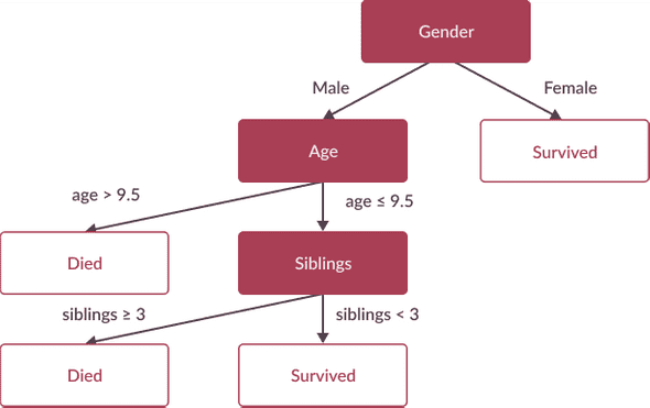
Decision Tree Learning is a commonly leveraged machine learning technique often utilized to generate a decision tree that can optimally predict the true values of target variables for observed individuals and items. In medicine, decision tree learning has been used to generate diagnosis predictions, in advertising, the technique is commonly used for identifying customer segments most likely to have particular demographic traits during market research, and in finance they have been used for predicting stock prices given the immense amount of information traders often have about a public company. Oftentimes, analyst’s will use Classification and Regression Trees (CART) as a primary algorithm for decision tree learning. The CART algorithm recursively splits observations into two subclasses in order to optimize a splitting criterion, a heuristic measuring the accuracy of predictions made given a particular split. Common splitting criteria used for CART are gini impurity and information gain, which both measure the probability that, given a particular split, an observed item on either side of the split is classified incorrectly. Consider another decision tree toy example presented below which aims to predict whether or not a passenger on the Titanic died or survived after it sank, given a set of information describing them. For this decision tree, which was learned by CART, the conditions defining branches of the tree, such as “siblings >= 3” or “age > 9.5” were chosen in order to optimize for the decision tree’s accuracy. The red nodes of this tree are splitting nodes representing the information used to separate passengers based on variables provided as input to the CART algorithm. The white nodes at the bottom of this tree are leaf nodes representing the information used to separate passengers based on variables provided as input to the CART algorithm.

Figure 4: An example of a decision tree learned using CART for the classification task of identifying which passengers on the Titanic survived after it sank. Utilizing this tree, and given information about the gender, age, and number of siblings of an individual passenger on the titanic, an analyst can acheive an estimate of whether it is more likely that the passenger survived or died.

Decision Tree Learning For Causal Inference

Decision tree learning is a very powerful technique for achieving high accuracy within the classification and regression problems it was designed to solve. If you’re interested in learning more, I would definitely suggest you read through this excellent blog post describing decision tree learning in greater depth . However, what does this have to do with causal inference? In my first blog post, I described causal inference tasks as separate from classification and prediction tasks, so how can decision trees help an analyst estimate heterogeneous treatment effects?

When an analyst uses decision tree learning for estimation of heterogeneous treatment effects, the entire process is typically different from those of decision tree learning for classification and prediction tasks. Decision trees used for these traditional inference tasks generally estimate a function mapping characteristics about individuals to the value of a target variable, such as the decision tree presented in Figure 4, which maps information about passengers on the Titanic to their probability of surviving its crash. Adversely, decision trees for causal inference are generally used to separate data into buckets, in order to enable a calculation estimating average treatment effects within each node. The process of decision tree learning for causal inference can be separated into a step for each of these tasks, commonly referred to as the splitting step and the estimation step respectively.

Splitting Step

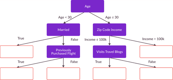
The splitting step of decision tree learning for causal inference consists of defining a set of rules for splitting observed individuals into buckets by values of variables defining their characteristics. This step generally consists of an algorithm similar to that of decision tree learning, which also aims to split observed individuals into groups given the values of variables describing their characteristics. However, in the splitting step of decision tree learning for heterogeneous treatment effect estimation, an analyst is not interested in estimating a particular value. To aid in understanding, one can think of this splitting step as very similar to the subclassification strategy for CATE estimation as discussed in my previous blog post. While subclassification generally consists of splitting observed individuals by arbitrary characteristics, such as their decade of birth as shown in Figure 1, the splitting step of decision tree learning for causal inference optimizes a subclassification strategy to maximize the accuracy of a subsequent average treatment effect estimation.

Figure 5: A learned decision tree which can be utilized to split observed individuals into buckets to solve my example airline digital advertising heterogeneous treatment effect estimation. Similar to the learned decision tree presented in Figure 4, this decision tree splits observed individuals by values of variables describing their characteristics. In this decision tree, the purple variables represent confounding variables conditioned on by the splitting step of this heterogeneous treatment effect process. The learned decision tree splits observed individuals by these characteristics in order to generate leaf nodes, which are empty and have a red border. The leaf nodes on this decision tree are red to show that they will be used to estimate the simple difference in means of the outcome variable Purchases Flight, and they are empty to illustrate that unlike in traditional decision tree learning, the leafs of this tree are not used to represent a value.

Estimation Step

The next step of Decision Tree Learning for causal inference, estimation, has no parallel in the process of decision tree learning. This step consists of leveraging the decision tree estimated in the splitting step and using the tree from that step to split observed individuals according to the defined rules. As a result of this splitting, each leaf of the tree will consist of a group of similar observed individuals exposed and unexposed to treatment. Thus, to estimate the effect of treatment on observed individuals within each leaf, an analyst must simply calculate the difference in mean outcomes between those that have been exposed to treatment and those that have not. This calculation, the simple difference in mean outcomes of observed individuals within each leaf, is an unbiased CATE estimation conditional on the values of variables which define the leaf (the conditional statements on the path from this leaf to the root node).

Below is an interactive visualization illustrating how the learned decision tree in Figure 4 can be used to estimate heterogeneous treatment effects. Observed individuals exposed and unexposed to treatment are recursively split into smaller and smaller subgroups and their outcomes are compared to achieve an estimate of heterogeneous treatment effects. The branches of this decision tree visualization are collapsable to illustrate the extent to which the number of exposed and unexposed observed individuals in a particular bucket decreases with the depth of the decision tree learned in the splitting step.

Ok, so we’ve identified a strategy for estimating heterogeneous treatment effects given a learned decision tree, that means we’re done right? It seems that all an analyst must do is use a decision tree learning algorithm, such as CART, to split observed individuals into homogeneous groups, and then calculate heterogeneous treatment effects at each leaf? Unfortunately, the application of a machine learning technique to a causal inference task is rarely that simple, and estimating heterogeneous treatment effects using decision trees is no exception.

Modifying CART For Causal Tree Learning

Unfortunately, CART and other traditional decision tree learning algorithms cannot be utilized in the splitting step of a heterogeneous treatment effect estimation. This is the case for two main reasons, one regarding CART’s splitting criterion and another regarding negative consequences of using the same observed individuals for calculations in the splitting and estimation steps. In the rest of this post, I will discuss Causal Tree Learning, a recently developed decision tree generation methodology designed specifically to mitigate CART’s pitfalls for heterogeneous treatment effect estimation. Causal tree learning modifies decision tree learning in two ways, in order to account for the shortcomings of CART which obstruct it from generating unbiased estimates of causal effects.

Splitting Criterion

The first aspect of CART that makes it incompatible for heterogeneous treatment effect estimation is its splitting criterion, or the heuristic the learning algorithm optimizes for when selecting splits for branching. Due to a few technical details regarding the estimation of heterogeneous treatment effects, this splitting criterion results in the generation of decision trees that are not consistent estimators, meaning that their estimated value of an optimal split does not converge to its true value, even when given an infinite amount of data. Consistency is a desirable property of a splitting criterion because it allows an analyst evaluate the expected accuracy of a calculated split, given the amount of observed individuals within their data set.

Additionally, just as causal tree learning for heterogeneous treatment effect estimation has a different aim than decision tree learning for prediction and classification, the splitting criterion for these processes must be different in order to optimize splits for their respective tasks. While the splitting criterion of CART optimizes for a decision trees accuracy in predicting the value of some target variable, the splitting criterion of a causal tree learning algorithm must optimize for two key heuristics.

• The first of which is balance between observed individuals in each leaf which are exposed and unexposed to treatment. Having approximately equal quantities of these two groups within each subclassification allows an analyst to accurately estimate differences in their outcomes, in order to calcuate an unbiased CATE estimation.
• The second key objective that a Causal Tree learning’s splitting criterion must incorporate is the expected accuracy of a CATE estimation made within a particular leaf. If leaves are not split in a way that cleanly separates groups of individuals with disparate outcomes, the accuracy of a resultant heterogeneous treatment effect estimation may significantly diminish.

Figure 7: A comparison between a leaf with poor balance and a leaf with good balance. The more uniform the number of observed individuals in a leaf exposed and unexposed to treatment, the more balanced that leaf is.

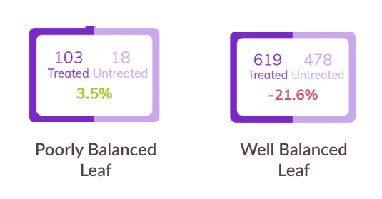
The Causal Tree learning algorithm fixes these issues by leveraging a modified splitting criterion as a heuristic for deciding optimal splits. Rather than leveraging traditional decision tree learning splitting criteria such as gini impurity and information gain, causal tree learning utilizes the expected mean squared error for treatment effects (written as $EMSE_\tau$) specified to apply directly to heterogeneous treatment effect estimation. In their paper, Athey and Imbens prove that this criterion is a consistent estimator, and thus $EMSE_\tau$ has the key statistical properties necessary for causal inference tasks. Additionally, they show that minimizing $EMSE_\tau$ corresponds with a multivariate optimization of two main objectives: the balance of exposed and unexposed observed individuals within each resulting leaf and the resulting accuracy of an estimation within each resulting leaf.

Honesty

Another challenge Athey and Imbens encountered when trying to design a decision tree learning algorithm which could be applied to heterogeneous treatment effect estimation, is overfitting, a phenomenon that occurs when a calculated estimation does not extrapolate well to a general population. When sampled data is used as input in the splitting step of decision tree learning for causal inference, splits are made to optimize for the accuracy of estimated treatment effects within each leaf. If that same data is used in a subsequent estimation step, the accuracy of a resultant CATE estimation may not generalize well to data outside of an analyzed sample, which has not been included in the calculation of said optimal splits.

Athey and Imbens resolve the overfitting problem by leveraging an estimation strategy known as honesty in the causal inference literature. At the beginning of a causal tree learning process the data measuring the characteristics and behaviors of observed individuals is separated into two subsamples, a splitting subsample and an estimating subsample.

• The splitting subsample is used in the splitting step of causal inference with decision trees and, as previously described, is leveraged to build a causal tree.
• The estimating subsample is used in the estimating step of causal inference with decision trees and, as previously described, this data is used to generate unbiased CATE estimates.

Figure 8: A depiction of the sample splitting process leveraged in Causal Tree Learning, "All Data" represents the entirety of data on observed individuals, which is separated into two subsamples.

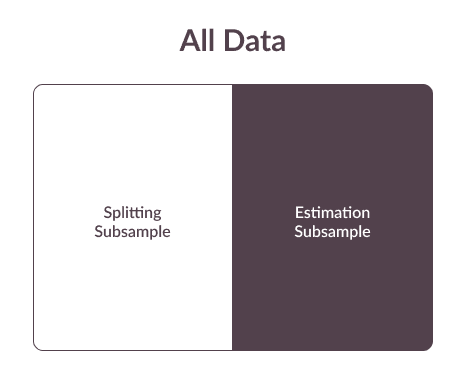
Honest tree learning is similar in nature to train test splits, commonly used to mitigate overfitting when evaluating supervised machine learning models for traditional inference tasks.

Causal Tree Learning And Its Applications

Figure 9: A comparison of the accuracy variety of techniques estimating heterogeneous treatment effects, displayed in Wager and Athey (2016) to illustrate the performance of causal trees for heterogeneous treatment effect estimation. This figure depicts a simulated causal effect, shown in the leftmost plot, that effects observed individuals heterogeneously over a two dimensional space. This leftmost plot depicts this simulated causal effect with a heatmap for which each color represents the quantity of the effect. The rightmost plot, depicts an effect estimated with a K-Nearest Neighbors Matching Algorithm, which was commonly used in causal inference and statistics before the invention of causal trees. The central plot depicts an estimation of this same effect calculated with Causal Trees. At a glance, it is easy to see the exceptional accuracy with which causal tree learning can estimate causal effects, when compared to the prior state of the art.

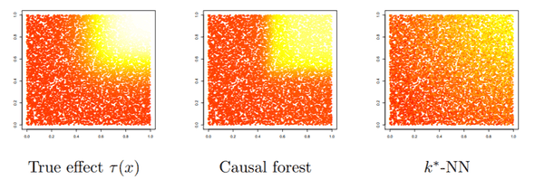
Athey and Imbens presented their modification of decision tree learning for causal inference in 2016 and since then there has been a Cambrian explosion of its application in industry and academia. Honest Causal Tree Learning has been implemented in R and Python and has been used extensively to understand the differential effects of a treatment, conditional on an expansive set of confounding variables. At the beginning of this post, I discussed the ways in which Causal Tree Learning has been used to solve causal inference tasks in a variety of business analytics scenarios,particularly for technology-enabled use-cases, such as personalized political messaging campaigns, search advertising optimization, and individualized medical treatment development utilizing large samples of clinical data. In my next blog post, I will present these practical applications of Honest Causal Forests in more detail, and I’ll discuss a set of methodologies an analyst can use to maximize the effectiveness of this machine learning technique for heterogeneous treatment effect estimation.