Confounding Bias

Why Is Causality So Hard?

In my previous posts, I’ve discussed methodologies for calculating causal effects in scenarios in which we observe an explanatory variable and an outcome variable and wish to quantify a causal relationship. In this simple scenario, one can use a calculation such as simple difference in mean outcomes to estimate average treatment effect (or use another estimation strategy to estimate another kind of treatment effect). However, I’ve also discussed how estimates can be biased, as a result of external factors affecting both an explanatory variable and an outcome variable. This bias is the main reason why causal inference tasks are so challenging and is why it has been a challenge to apply machine learning techniques to these tasks, until recently. Identifying and eliminating biases of estimated causal effects is the main concern of causal inference practitioners in business and academia, and the formalized strategy for describing such bias, which I discuss in this post, undergirds the majority of causal inference literature.

Causal Inference Obstacles In A/B Testing

Figure 1: Two variations of a button design which can have an effect on a user's propensity to place an order. A UX designer may suspect that changing the "Add to Cart" button's design from being in-line with a product description (left) to being fixed at the bottom of a mobile screen (right) will allow users to make more "impulsive" shopping decisions, causing them to add more products to their cart.

Consider the following structural causal model, describing a causal relationship between the display of a specific “Add To Cart” button design and a user’s decision to add a particular item to their cart, as presented in my previous post about average treatment effects. As previously mentioned, models similar to this are commonly used for analysis tasks in product design and marketing, when companies run A/B tests to determine the effect of a new feature on user behavior. The structural causal model is comprised of 3 observed variables, an explanatory variable describing the particular button design displayed to a user, labelled as Button Design ($\color{#7A28CB}B$) another explanatory variable describing the product which is shown to the user, labelled as Product Shown ($\color{#7A28CB}P$) and an outcome variable measuring whether or not a user adds an item to their cart, labelled as Adds to Cart ($\color{#EF3E36}A$). In order to focus our attention to an individual causal effect, the effect I’m interested in estimating $\textcolor{#7A28CB}{B} \leftarrow f_i(\textcolor{#7A28CB}{P})$ is marked with blue.

$\textcolor{#7A28CB}{B} \leftarrow f_i(\textcolor{#7A28CB}{P})$

$\textcolor{#EF3E36}{A} \textcolor{#7FB9E9}{\leftarrow f_i(}\textcolor{#7A28CB}{B}, \textcolor{#7A28CB}{P}\textcolor{#7FB9E9}{)}$

The corresponding causal graph of this structural causal model, with our causal effect of interest once again marked with blue, is as follows.

Figure 2: The structural causal model describing Product Shown's effect on Button Design and Adds To Cart. For a particular user, the particular product they see when browsing an e-commerce site can effect their decision to add the item to their cart. Additionally, if due to engineering requirements we need to fix one button design to each product page, the product which is shown to a user effects the button design which the user sees.

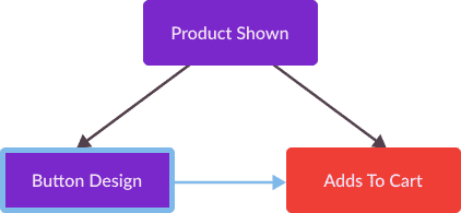
As a result of the presence of Product Shown, we cannot estimate the extent to which a particular button design effects a user’s decision to add a product to their cart simply by analyzing how different users react to different button designs. For example, a rare good that is frequently out of stock, such as highly demanded dumbbells might be added to cart with much higher likelihood than a luxury good which users only view when browsing styles. If a in-line block button design is displayed with dumbbells, while a fixed button design is displayed with a luxury items, then users may be more likely to add items to their cart for an in-line block button design, for reasons external to its UX.

Figure 3: Mockup of the products users might see on an E-commerce site with differing designs. If we randomly assign users one of these two "Add To Cart" button designs, it is possible that individual users will see different products and their measured treatment effect may vary as a result of Product Shown rather than Button Design.

As a result of the Product Shown’s effect on both Button Design and Adds to Cart, an analyst cannot calculate an estimate of causal effects between these latter two variables solely from observations measuring individual responses to various button designs. In causal inference literature a variable like Product Shown, which has an effect on both an explanatory and outcome variable of interest is known as a confounding variable. The bias resulting from the presence of a confounding variable, which obscures estimation of specific causal effects, is known as confounding bias.

When confounding variables has an effect on both variables in a causal relationship of interest, the explanatory variable is associated with an outcome variable due to factors other than purely causal effects. For structural causal models which exhibit confounding bias between a particular explanatory variable ($\color{#7A28CB}X$) and outcome variable ($\color{#EF3E36}Y$), an individual’s measured explanatory variable $\color{#7A28CB}X_i$ is not independent from their potential outcomes, a statement formally presented with notation below. Here, we use a generalized notation for a set of potential outcomes $\color{#EF3E36}Y_x$, rather than $\color{#EF3E36}Y^0$ and $\color{#EF3E36}Y^1$, in order to represent scenarios for which we can observe more than 2 potential outcomes corresponding to more than 2 values of explanatory variable $\color{#7A28CB}X$.

$\textcolor{#EF3E36}{Y_x}\not\!\perp\!\!\!\perp \textcolor{#7A28CB}{X}$

Recall from my previous post, that when we try to use the simple difference in mean outcomes to estimate average treatment effects on an outcome variable, our resultant estimate is biased when potential outcomes are not independent from measured values of an explanatory variable. Confounding bias obscures the SDO for ATE estimations, as it does for a variety of estimators designed to estimate many kinds of treatment effects. As a result, eliminating confounding bias is the main focus of a great deal of causal inference literature.

Eliminating Confounding Bias, Achieving Independence

Remember that mathematically, “eliminating confounding bias” consists of ensuring independence between the potential outcomes $\color{#EF3E36}Y_x$ of an observed individual and the corresponding value of an explanatory variable $\color{#7A28CB}X_i$, as if no confounding variable were present. If Product Shown did not have an effect on Button Design and Adds to Cart correlating the two variables, such an independence assumption would hold without any modification to calculated effects. Is there a way we can “account” for this confounding variable, in order to eliminate their resultant bias?

Fortunately, yes! Often times, even when an explanatory variable and a set of potential outcomes are not independent, they will be conditionally independent with respect to some set of confounding variables $\color{#7A28CB}Z$, meaning that $\color{#7A28CB}X$ and potential outcomes $\color{#EF3E36}Y_x$ are independent as long as the variables in $\color{#7A28CB}Z$ are held constant. This statement is formally written as

$\textcolor{#EF3E36}{Y_x}\!\perp\!\!\!\perp \textcolor{#7A28CB}{X}\ |\ \textcolor{#7A28CB}{Z}$

If an explanatory variable and an outcome variable are conditionally independent, we can calculate an unbiased estimate of causal effects by only measuring causal effects for which all variables in $\color{#7A28CB}Z$ are held constant. This technique for eliminating confounding bias is known as controlling for confounding variables. For example, suppose the structural causal model describing the hypothesized relationship between Button Design and Adds To Cart, contains an additional statement.

$\textcolor{#EF3E36}{A_x}\!\perp\!\!\!\perp \textcolor{#7A28CB}{B}\ |\ \textcolor{#7A28CB}{P}$

Expressing that Button Design and Adds To Cart are both conditionally independent to Product Shown. This implies that if I chose to fix product shown and show every user the same product while varying designs of an “Add To Cart” button, I can achieve an unbiased estimate of treatment effects using a method such as the simple difference in mean outcomes, as described in my previous post.

A Generalized Approach

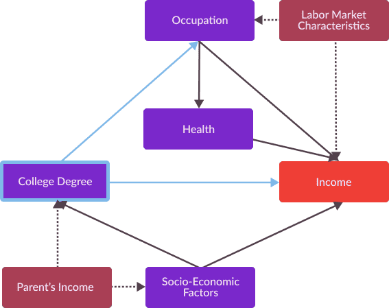
Ok, it seems simple enough to hold a single variable constant within an experiment in order to estimate causal effects ceteris paribus (which is Latin for all else equal). However, how can we extend this strategy to analysis in observational settings, for which we cannot hold confounding variables “constant”, or any other variables for that manner? What should we do as causal diagrams become large as well as the number of confounding variables? For example, consider the following more complex causal graph

Figure 4: Causal graph representing the structurucal causal model for estimating the causal effect of college on wages from Chapter 3 of Mostly Harmless Econometrics by Angrist and Pishke ¹. This diagram illustrates the variety of factors that can bias an estimate of this causal effect. For example, for very wealthy people, college may be more accessible as is getting a high income job, so a high correlation between having a college degree and having a high income does not necessarily imply the causal effect of a College Degree on Income is particularly large.

How can we formalize a set of strategies for controlling for confounding variables in order to accurately estimate causal effects? Well in 1995, Turing Award winning computer scientist Judea Pearl wrote Causal diagrams For Empirical Research which leveraged analysis of causal graphs to do just this ². In this paper, he presented two “adjustments” which can be made to measurements of causal effects in order to control for the confounding bias when analyzing structural causal models. These two adjustments are back door adjustments and front door adjustments named after the graph structures required for them to be leveraged.

First, Some Terminology

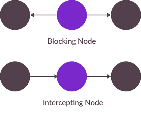
In my discussion of the causal graph structures leveraged to develop a formal methodology for eliminating causal bias, I will use two terms from graph theory to reference two types of 3 node substructures. These terms are blocks and intercepts. A node blocks a path between two nodes if it has two out-edges on the path, each in the direction of its starting and its ending node. A node intercepts a path between two nodes if it has one out-edge and one in-edge on the path, with the out-edge and the in-edge in the direction of the path’s ending node. Below is a figure illustrating these definitions.

Figure 5: A figure illustrating a blocking and an intercepting node (purple) on the path between a starting and an ending node (brown).

Back-door Adjustment Criterion

When describing the conditions necessary for eliminating confounding bias, causal inference practitioners often leverage graph theoretical concepts commonly applied to directed acyclic graphs. The first of these are back-door admissible sets. Given a pair of an explanatory and an outcome variable ($\color{#7A28CB}X$,$\color{#EF3E36}Y$) as well as a causal graph, a set of edge is back-door admissible if it blocks every path $\color{#7A28CB}X$ and $\color{#EF3E36}Y$ in the causal graph, excluding effects caused by $\color{#EF3E36}X$. Effects caused by $\color{#7A28CB}X$ are the causal effects we are interested in estimating and any other blocked path from $\color{#7A28CB}X$ will consist of confounding variables obscuring the estimation. Hence, identifying these confounding variables is a primary concern for causal inference practitioners.

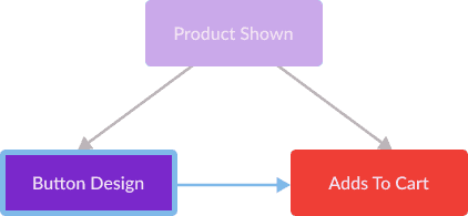
For example, in the causal graph describing the effect of an “Add To Cart” button on a users propensity to add a particular item to their cart, we can separate out a back-door admissible set as follows.

Figure 6: Causal graph analyzed for estimating average treatment effects with A/B testing for which the unique back-door admissable set for Button Design and Adds To Cart is transparent, while variables and relationships not included in the set are opaque. Note that the only variable blocking all paths from Button Design to Adds To Cart (our causal effect of interest) is Product Shown, this variable comprises a back-door admissible set.

In the more complex causal graph I previously presented describing the effect of education on wages, we can identify a set of variables $\color{#7A28CB}Z$ that is back-door admissible.

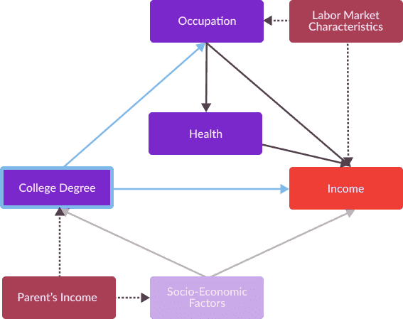Figure 7: Causal graph analyzed for estimating the effect of a college degree on an individual's lifetime earnings for which the unique back-door admissable set for College Degree and Income is transparent. Since, the only node that blocks paths from College Degree to Income that is not our causal effect of interest is Social-Economic Factors, this variable comprises a back-door admissible set.

We can use back-door admissible sets to make a particular explanatory variable independent from its corresponding potential outcomes. The back-door adjustment criterion provides a methodology for ensuring that $\color{#EF3E36}Y_x$ and $\color{#7A28CB}X$ are conditionally independent, enabling estimation of a causal effect from an explanatory variable to an outcome variable. This criterion states: if the set of variables $Z$ is back-door admissible relative to explanatory and outcome variables ($\color{#7A28CB}X$, $\color{#EF3E36}Y$), then

$\textcolor{#EF3E36}{Y_x}\!\perp\!\!\!\perp \textcolor{#7A28CB}{X}\ |\ \textcolor{#7A28CB}{Z}$

Back-door adjustment causal inference strategies are those which hold variables of a back-door admissible set constant, while varying explanatory variables to measure their effect on outcome variables. The most commonly used causal inference strategies in fields such as economics and product design are “back-door adjustment” causal inference strategies. For example, one technique I could leverage to maximize insights from my A/B test would be to show all users the same product, in order to control for Product Shown. If I wanted to estimate average treatment effects of my new button design for all shoppers regardless of the product, I could’ve also A/B tested my “Add To Cart” button across the whole website and compared causal effects measured in different product categories, using a process known as matching. This would entail identifying product categories I believe should yield different responses from individual users, and estimating the causal effect of different button designs by calculating causal effects between individuals within the same product category. For example, I could aggregate measured behavior from individuals buying video games in order to identify a matched observation and weight this observation by the proportion of sessions in which a user browses a video game product page when calculating a total average treatment effect.

If my causal graph were more complex and had an unmanageably large number of confounding variables, I could collapse these variables with logistic regression into a single variable (known as a propensity score) and “match” individual observations of Button Design and Adds To Cart with values of this score. A diagram describing how these variables can be collapsed is shown below.

Figure 8: Causal graphs showing how we can reframe our model so we can "collapse" a variety of confounding variables into a Propensity Score, which in this case estimates a user's propensity to add a good to their cart regardless of their button design. In the first diagram, we model 5 additional explanatory variables which have an effect on both Button Design and Adds To Cart. For this model, these 5 variables comprise a unique back-door admissible set, so to identify our causal effect of interest we would need to control for all of them. In the second diagram, we reframe our model such that only the Propensity Score comprises a back-door admissible set, allowing us to identify treatment effects by estimating this single variable.

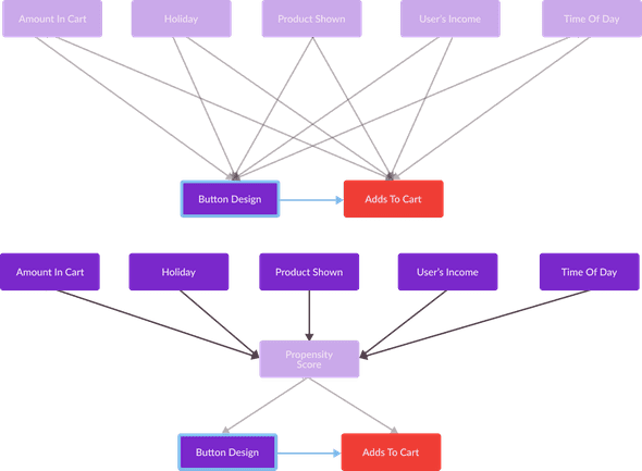
I will cover this technique, known as propensity score matching, in more detail in future blog posts.

Front Door Adjustments

Another type of adjustment we can make when eliminating confounding bias from an estimation of causal effects is a front-door adjustment which adjusts for a set of confounding variables $\color{#7A28CB}Z$ using additional information about a set of mediator variables $\color{#7A28CB}M$, rather than by controlling for the confounding variables. A mediator variable is a variable which is affected by an explanatory variable $\color{#7A28CB}X$ of interest, and also has an effect on $\color{#EF3E36}Y$ “through the front door”. Front-door adjustments can be made as a result of the front door criterion. Given an explanatoy variable $\color{#7A28CB}X$, a set of confounding variables $\color{#7A28CB}Z$, and an outcome variable $\color{#EF3E36}Y$, a set of variables $\color{#7A28CB}M$ satisfies the front-door criterion if

1. The variables in $\color{#7A28CB}M$ intercept all paths from the explanatory variable $\color{#7A28CB}X$ to the outcome variable $\color{#EF3E36}Y$.
2. No confounding variable in $\color{#7A28CB}Z$ has an effect on any of the mediator variables in $\color{#7A28CB}M$
3. All paths from the mediator variables in $\color{#7A28CB}M$ to the outcome variable $\color{#EF3E36}Y$ are blocked by an explanatoy variable $\color{#7A28CB}X$ and the set of confounding variables $\color{#7A28CB}Z$

The set of variables in $\color{#7A28CB}M$ which satisfy the front-door criterion, are known as mediator variables, this term comes from the field of psychology, in which measurement of mediator variables are used to explain how external physical events effect an individuals psychological state. An example of a set of mediator variables $\color{#7A28CB}M$ which satisfies the front door criterion with respect to an explanatory variable, an outcome variable, and a set of confounding variables is shown below.

Figure 9: Causal graph including a set of mediator variables which satisfy the front-door criterion. Note that the two mediator variables intercept the blue path between the explanatory variable and the outcome variable, that no confounding variable has an effect on a mediator variable and that each mediator variable has only one path from each mediator variable to the outcome variable. Thus, the two mediator variables in this causal graph satisfies the front-door criterion.

When a set of variables satisfies the front-door criterion, with respect to an explanatory variable and an outcome variable which are affected by confounding bias, we can calculate an unbiased estimate of a causal effect between the two variables with the following procedure, commonly known as a front door adjustment in causal inference literature.

1. Estimate the effects of the explanatory variable $\color{#7A28CB}X$ on the mediator variables in $\color{#7A28CB}M$, This can be done without controlling for any variables, as there is no confoudning variable with an effect on both of these variables.
2. Estimate the effects of all mediator variables in $\color{#7A28CB}M$ on the explanatory variable $\color{#7A28CB}Y$. The set of confounding variables $\color{#7A28CB}Z$, has an effect on both $\color{#7A28CB}M$ (through the explanatory variable $\color{#7A28CB}X$) and outcome variable $\color{#EF3E36}Y$ and thus this estimation will be distorted by confounding bias. However, we can adjust for this confounding bias by controlling for explanatory variable $\color{#7A28CB}X$, as this single variable satisfies the back-door criterion (shown in the bottom image of the figure below).
3. Once we have estimated the effect of the explanatory variable $\color{#7A28CB}X$ on the mediator variables in $\color{#7A28CB}M$ and the effect of the mediator variables in $\color{#7A28CB}M$ on outcome variable $\color{#EF3E36}Y$. We can take the product of these two estimated causal effects in order to calculate an estimate for the causal effect of explanatory variable $\color{#7A28CB}X$ on outcome variable $\color{#EF3E36}Y$.

For example if the causal effect, we were interested in estimating were the average treatment effect of individual observations of $\color{#7A28CB}X$ on $\color{#EF3E36}Y$, with a single mediator variable $\textcolor{#7A28CB}{M}$ and a single confounding variable $\color{#7A28CB}{Z}$, we would estimate $ATE_{\textcolor{#7A28CB}{X} \rightarrow \textcolor{#7A28CB}{M}}$ (controlling for $\textcolor{#7A28CB}{X}$), as well as $ATE_{\textcolor{#7A28CB}{M} \rightarrow \textcolor{#EF3E36}{Y}}$ to produce the following estimation:

$ATE_{\textcolor{#7A28CB}{M} \rightarrow \textcolor{#EF3E36}{Y}} = ATE_{\textcolor{#7A28CB}{X} \rightarrow \textcolor{#7A28CB}{M}} \times ATE_{\textcolor{#7A28CB}{M} \rightarrow \textcolor{#EF3E36}{Y}}$

Causal graphs, highlighted to illustrate the process of a front-door adjustment are provided below.

Figure 10e: Figure showing the two causal effects calculated when completing a front door adjustment, the causal graph at the top highlights the causal effect estimated of the explanatory variable on the mediator variable and the causal graph at the bottom highlights the causal effect of a mediator variable on an outcome variable. The explanatory variable in the bottom causal graph is transparent to represent that it comprises of a back-door admissible set for the mediator variable and outcome variable and thus can be controlled in order to calculate an unbiased estimate of the causal effect between these two variables.

Mediator variables, as their name implies, are often considered to “mediate” a causal relationship of an explanatory variable on an outcome variable. For example, suppose that I discovered that the causal effect of Button Design on Adds To Cart was indirect, and that there existed a mediator variable that mediates their relationship. Perhaps, it is not actually a fixed button design which makes users more likely to add an item to their cart, but rather the fixed button design causes a user to spend less time on the page for a particular product, and the less time a user spends on the page for a product, the more likely they are to make an impulsive decision to add the product to their cart. In this scenario, Time Spent On Page is a mediator variable, satisfying the front-door criterion for an explanatory variable Button Design, a confounding variable Product Shown, and an outcome variable Adds To Cart. Thus, we can use a front door adjustment to calculate the causal effect of Button Design on Adds To Cart.

Figure 11: Figure showing the two causal effects which must be calculated in order to achieve an unbiased estimate of Button Design on Adds To Cart.

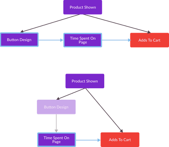
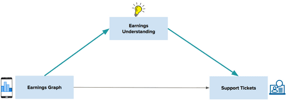
Front-door adjustments are a powerful causal effect estimation technique that build upon the utility of back-door adjustments. Note that, in the estimation of the effect of Button Design on Time Spent On Page, as well as the controlled estimation of the effect of Time Spent On Page on Adds To Cart, I never incorporate the confounding variable Product Shown into my calculations. In general, front-door adjustment techniques do not require observed confounding variables in order to eliminate confounding bias. For this reason, front-door adjustment techniques can be especially powerful for solving a variety of causal questions, as they allows us to estimate causal effects when confounding variables are unobserved. Front-door adjustment techniques are commonly used in genetics, for example, the statistician Azam Yazdani used the front-door criterion to identify the effects that ethnicity has on the blood glucose level of a population, given BMI and a variety of other health metrics. Front-door techniques have also been used in fields outside of the life sciences, the sociologist Otis Dudley Duncan used the front-door criterion to estimate how an individual’s age and date of birth affects their respect for their elders. More recently, Uber has used mediation modeling to identify the most influential mediator variables which intercept the causal effect of a new driver app design on a rider’s propensity to file a ticket. Identifying and measuring these mediator variables, helps Uber break down causal effects between an explanatory variable and an outcome variable which may be impacted by unmeasured confounding variables.

Figure 12: Image from Uber's blog post on the applications of mediation modelling. Uber redesigned their Earnings Graph for drivers in 2018, and sought to understand the mechanism by which this change incurred a decrease in the support tickets filed due to a driver's misunderstanding of their earnings for a given week. They found that earnings understanding, measured using a short survey sent out to drivers, was a signficant enough mediator variable to be used for front-door criterion adjustments, leveraging a technique known as mediation modelling. I will cover mediation modelling in more detail in a future post.

What’s Next?

Now that I’ve formalized a description of confounding bias, the main obstacle for causal effect estimation, and formalized a taxonomy of strategies for identifying and eliminating this bias, I can dive deeper into specific back-door and front-door adjustment strategies. Particularly, I can begin to describe the machine learning methodologies commonly used for extracting causal inference insights and in future posts, I will discuss the utility of these methodologies for solving a variety of causal inference problems. Now that I have described the basic tenets of the vast scholarship on causal inference, I can go more in depth in my discussion of the causal inference techniques which can help business analysts understand exactly how much their interventions effect their user’s behavior, unlocking latent value from an expanse of under-utilized data.