Propensity Score Matching
June 17, 2020
Hey! This post references terminology and material covered in previous blog posts. If any concept below is new to you, I strongly suggest you check out its corresponding posts.
Confounding Bias
June 10, 2020So far, our discussions of causality have been rather straightforward: we've defined models for describing the world and analyzed their implications. In this post I present the obstacles we may face when leveraging these models as well as the 'adjustments' we can make to remove them.
Estimating Average Treatment Effects
June 07, 2020When quantifying the causal effect of a proposed intervention, we wish to estimate the average causal effect this intervention will have on individuals in our dataset. How can we estimate average treatment effects and what biases must we be wary of when evaluating our estimation?
In my previous post, I presented a rigorous definition for confounding bias as well as a general taxonomy comprising of two sets of strategies, back-door and front-door adjustments, for eliminating it. In my discussion of back-door adjustment strategies I briefly mentioned propensity score matching a useful technique for reducing a set of confounding variables to a single propensity score in order to effectively control for confounding bias 1. Propensity score matching is a quite powerful, rather straightforward backdoor adjustment technique typically used in the presence of selection bias or bias arising from differences between those who are selected to receive treatment and those who are not. Propensity score matching can be used in marketing to estimate a “lift” in revenue due to a particular digital advertising campaign, in medicine to identify the precise effect that smoking has on a variety of health outcomes, and in economics to measure the benefits of socioeconomic support programs in the US. In this blog post and the next, I will present a detailed set of steps for leveraging propensity score matching in order to effectively eliminate confounding bias from a large set of variables.
Another Kind Of Lift
Suppose, I’ve decided to start a direct-to-consumer athletic equipment company (which would be a great business around the time of writing this). Particularly, I am interested in building a brand around selling dumbbells to athletic enthusiasts, looking to build a complete home gym. One insight I intend to use to maximize the ROI of my marketing spend, is to purchase youtube ads targeting fans of professional weightlifters, and frequently watch weightlifting competitions such as World’s Strongest Man on Youtube. I believe that running a widespread campaign targeting these weightlifting fans will net me a great deal of revenue, but want to measure the effect of such a campaign on purchases, to make sure I don’t spend the little funding I have on an expensive marketing campaign with lackluster results.

Precisely, I’m interested in measuring the increase in sales I should expect as a result of my digital advertising campaign, commonly called lift by quantitative marketers. Currently, I can use browser cookies to track the individuals who view my ad, and the individuals who visit my website to purchase my products. A naïve solution, may be to simply measure the number of individuals who purchase products on my site shortly after seeing an ad, dividing this by the total number of individuals who saw my ad, and assuming this value to be the average treatment effect of my marketing campaign. For example, if 100,000 people saw an ad from my campaign, and 1,000 of those individuals subsequently made a purchase on my site, I might (naively) state that exposure to my campaign makes an individual 1% more likely to buy a dumbbell from my company, given how expensive dumbbells are, that’s a pretty good ROI!
Unfortunately, as is common with causal inference tasks, it’s not quite that simple. The individuals who watch weightlifting youtube videos are athletics fanatics, many of whom are on the hunt for sites with high quality equipment in stock. Some of these consumers are probably very likely to purchase a good from my site, regardless of whether or not they see my Youtube ad. For this reason, I cannot be sure how much of an effect I can attribute to my ads, as they are not the sole factor driving purchasing decisions. In this scenario, athletic enthusiasm is a confounding variable as discussed in my previous post. Athletic enthusiasm has an effect on the probability that a user is exposed to an ad as well as on the probability that an individual consumer purchases a product from my site. Thus, in order to be confident in my estimate of the effect my ads have on individual purchasing decisions, I need to be sure I have eliminated all confounding bias distorting my calculations. Unfortunately, “athletic enthusiasm” is an unmeasurable concept, it’s not immediately clear which metrics I should look at to quantify “enthusiasm” for athletic activity. Is there a way I can use the data I do have in order to eliminate confounding bias?
Causal Graphs In Digital Advertising
As is common in analysis causal inference tasks, the first step of our analysis is to draw the causal graph representing the interacting processes we wish to measure. The main explanatory variables we are analyzing for this task are as follows:
Watches Weightlifting: Measuring whether or not individual consumers watch weightlifting youtube videos. My brands ads are only played against such youtube videos, so understanding the factors influencing this variable is crucial for my analysis.
Exposed To Ad: Measuring whether or not an individual was exposed to an ad from my brand.
Much like many popular digital advertising offerings, Youtube gives me access to anonymized data describing a variety of characteristics of consumers who are exposed and unexposed to my advertising campaign. Many of these variables are useful for my analysis, as they have an effect on the likelihood that an individual watches weightlifting as well as the likelihood that they make a purchase on my site. These variables are:
- Past Behavior: Data measuring the behavior on Youtube of an individual consumer. This includes information such as previous engagements with my brand, generalized information about viewing history, and data detailing a consumer’s how often a user clicks through an ad.
- Demographic Data: Data measuring groups individual consumers belong to, such as their zip code, gender, or age.
- Psychographic Data: Data conducted from surveys measuring the interests, values, and personalities of consumers who may see my ad.
Measurements of all these explanatory variables can be leveraged to estimate their effect on the following outcome variable:
- Buys Dumbell: Measuring whether or not an individual buys a dumbbell within a week of seeing an ad.
The causal graph relating all of these variables is as follows.
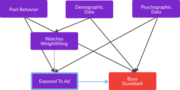
Recall from my previous post, that one way we can eliminate confounding bias that affects our estimation of causal effects is to identify a set of variables which satisfy the back door criterion for Watches Weightlifting and Buys Dumbbell , and then compare Exposed To Ad and Buys Dumbbell with these variables held constant. Using the definition of backdoor admissible provided in my previous post, we can separately identify a unique backdoor admissible set as follows.
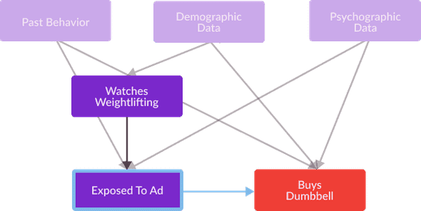
Identifying confounding variables and holding them constant may get us a slightly better estimate, but for this use case, such a technique can pose a variety of challenges. My confounding variables (Past Behavior, Demographic Data, and Psychographic Data) are very high dimensional and consist of many individual scalars, and controlling for so many scalars can adversely affect the accuracy of my estimate. To control for a large number of confounding variables, we need a very large sample size to get an accurate estimate of their effect on Explanatory Variables and Outcome Variables. Thus, in order to effectively control for this expanse of background information, analysts often prefer to reduce its dimensions into one scalar and then measure causal effects holding this scalar constant. A particularly useful reduction for this task is the estimation of a propensity score, which measures the probability that an individual is exposed to a particular treatment, such as selection for a medical trial or engagement with a marketing campaign. In this definition, exposed to treatment means the same thing as “treated” used in previous blog posts, however I use the former terminology to communicate that analyst’s do not control which individuals are treated in settings which require propensity score matching (if an analyst did, they could assign treatment randomly, such that no variable affected the explanatory variable in their causal relationship of interest, thus confounding bias would not be a problem).
The main challenge of causal effect estimation in the presence of confounding variables is the effect these variables have on an individual’s probability of exposure, as well as, their effect on any outcome variables of interest. Reframing a structural causal model, to accent this probability can be a powerful technique for identifying unbiased estimation strategies. A causal graph illustrating this “reframing” for my digital advertising causal inference task is presented below. In this example, a consumer’s propensity score can be interpreted as a quantitative estimate of the “athletic enthusiasm” which inspires them to watch a weightlifting youtube video, and to be subsequently exposed to my ads.
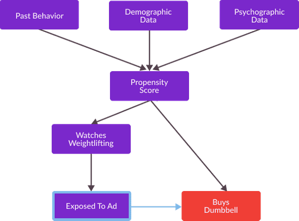
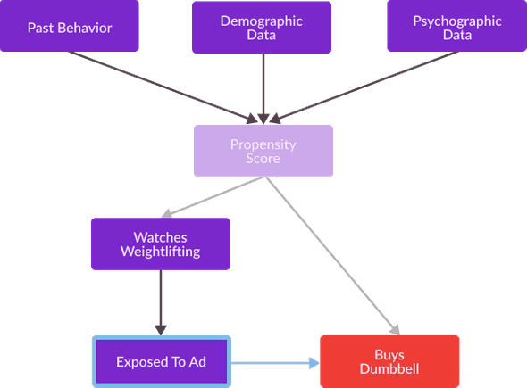
For this causal graph, the confounding variable Propensity Score comprises a backdoor admissible set. Thus, Exposed To Ad and Buys Dumbbell are conditionally independent given an individual’s Propensity Score. As mentioned in my previous post, this means that we can calculate an unbiased estimate of Exposed To Ad’s effect on Buys Dumbbell comparing the purchasing decisions of individuals with the same Propensity Score.
Calculating A Propensity Score
Ok, so in order to analyze this causal effect, one may want to estimate a propensity score, measuring the probability that an individual consumer is exposed to one of my ads. How can an analyst even calculate such an estimate? Well, when complete inference problems focused on estimating probabilities, it is standard for analysts to use logistic regression to generate a model for calculating a propensity score. Particularly, an analyst is interested in fitting a vector of confounding variables for each individual to an indicator variable (which is 1 if an individual is exposed to treatment and 0 if they are not). The logistic regression for propensity score calculation fits a function of the following form:
For example, the logistic regression of exposure to one of my ads on a single confounding variable, age, is as follows.
Logistic Regression of Age On Exposure to My Ads
Once an analyst has completed a logistic regression estimating the relationship between a set of confounding variables on the probability of exposure to a particular treatment, their derived model can be used to calculate a propensity score for each individual they observe. Below is a plot displaying the propensity scores I’ve calculated for each individual I can observe from the data provided by my digital advertising campaign. For each of the 32 displayed individuals a propensity score was calculated from Past Behavior, Demographic Data, and Psychographic Data. Sample IDs are then assigned to individuals sorting them by their propensity score.
Observed Individuals By Calculated Propensity Score
Matching Propensity Scores
Ok, so once an analyst has calculated the propensity scores for each observed individual, what do they typically do next? What’s the best way we can control for this variable, or hold it constant, in order to produce an unbiased estimate of a particular causal effect? When leveraging propensity score matching for causal inference tasks, matching refers to the process of identifying groups of individuals with similar propensity scores and comparing the values of their corresponding outcome variables in order to estimate a causal effect. Within these groups, called matched samples, propensity score is constant across individuals, and thus we can compare the different outcomes between exposed and unexposed individuals while holding propensity score constant 2.
For example, consider the interactive visualization below displaying the propensity score matching process for my digital advertising causal inference task. This visualization at first displays the same plot shown in figure 7, of 32 individuals sorted by their propensity score. After pressing the “Match Observations” button, datapoints representing similar propensity scores will match, represented by a migration to a plot of matched samples. We can produce an unbiased estimate of causal effects by comparing differing outcomes for the individuals with similar propensity scores in each matched sample.
Matched Samples By Estimated Propensity Score
Algorithms used to match individuals with “similar” propensity scores are called matching algorithms. Analysts are free to select from a variety of such algorithms, in order to generate a match that fits their particular needs. Some matching algorithms are optimal matching algorithms, and identify a set of matches which minimize the total distance between individuals in every match. Greedy matching algorithms are much faster than optimal matching algorithms and can be used on much larger datasets, however they produce matched observations that are not optimally similar. An analyst’s choice of matching algorithm is crucial to the utility of a propensity score match, as the “quality” of the match, or the average similarity between matched individuals, is a consequential factor in the accuracy of estimated causal effects.
Greedy vs. Optimal Matching Algorithm Comparison
In notation, we represent an exposed sample ’s’ match with a similar “unexposed” sample with . For example, the values of an outcome variable of a match between an arbitrary exposed individual and an unexposed individual can be represented as follows:
Likewise, represents the difference in outcomes between an exposed and an unexposed individual in a matched pair. For my digital advertising causal inference task represents the difference in outcomes between two matched consumers. This value is an unbiased estimate of the causal effect of my advertisements on the purchasing decisions of individual , as and have such similar propensity scores that my backdoor admissible set (which consists solely of Propensity Score) has successfully been held constant.
Calculating An Effect
Once an analyst has matched their observed individuals by similarity, producing an estimate of their causal effect of interest is actually quite straightforward. If we wished to estimate an average treatment effect, a quantification of a causal effect discussed in a previous blog post, we can take the average of for each exposed individual in order to estimate the average difference in outcomes between treated and untreated individuals. For my digital advertising task, concerned with estimating the effect that exposure to my ads has on purchasing decisions, the average of represents the “lift” of my advertising campaign. Below is a table detailing this calculation for the individual consumers I observed and matched.
| Matched Sample ID | Avg. Propensity Score | |||
|---|---|---|---|---|
| 0 | 0.03 | 0 | 0 | 0 |
| 1 | 0.14 | 0 | 1 | 1 |
| 2 | 0.25 | 1 | 1 | 0 |
| 3 | 0.33 | 0 | 0 | 0 |
| 4 | 0.49 | 1 | 1 | 0 |
| 5 | 0.68 | 0 | 0 | 0 |
| 6 | 0.81 | 0 | 1 | 1 |
| 7 | 0.94 | 0 | 1 | 1 |
| Avg. | 0.46 |
Assuming my match is not afflicted with any statistical challenges, my estimated “lift” is or 37.5%. With this calculation, as well as the prices of dumbbells typically bought from my store, I can precisely understand the revenue generated when an individual consumer sees one of my ads, and adjust my marketing spend accordingly.
Obstacles And Opportunities Of Propensity Score Matching
Well my problem has been solved! After calculating a propensity score for each individual observed consumer, matching consumers with similar propensity scores, and calculating the difference in outcomes between individuals within the same match I was able to effectively control for confounding bias which may have distorted an estimate of Exposed To Ad’s effect on Buys Dumbbell.
However, some healthy skepticism of the utility of this technique is certainly warranted. After all, causal inference tasks are rarely quite that simple in the execution of causal inference tasks. Are there any pitfalls I should be concerned about as I utilize this estimate to make data-driven digital marketing decisions? More generally, what obstacles to estimation accuracy should an analyst be wary of when interpreting analysis from a propensity score match? What opportunities do more scalable modelling techniques from machine learning literature present for overcoming these obstacles? I will discuss all this and more in my next Causal Flows post! Stay tuned and be sure to subscribe to receive email alerts for future posts.