As discussed in my previous blog post, propensity score matching is a powerful technique for reducing a set of confounding variables to a single propensity score, so an analyst can easily eliminate all confounding bias. In that post, I described a scenario in which a marketer may struggle to identify the causal effect of a particular campaign, and discussed a rigorous causal inference technique built to solve this problem. Specifically, I provided a simple procedure for estimating propensity scores, matching individuals based on this estimation, and calculating a measurement of a causal effect by comparing observed individuals within the same match. In this post, I will describe a set of challenges an analyst should be wary of when attempting to estimate a particular causal effect with propensity score matching. Many of the challenges I will discuss in this post are common across a variety of causal inference techniques so analyzing these vulnerabilities for propensity score matching, a relatively simple procedure can help an analyst build an intuition of what to look out for when evaluating causal inference techniques.

As is common with many causal inference techniques, an analyst must be cautious when estimating a causal effect using propensity score matching. While propensity score matching is a powerful way to control for confounding variables in order to calculate an unbiased estimate of a causal effect, there are a variety of challenges an analyst must be cautious of, as they may diminish the accuracy of their estimate. These challenges, which threaten the efficacy of a particular estimation method are referred to in causal inference literature as threats to external validity. In the presence of a threat to external validity, in an external scenario in which an intervention is applied, the observed causal effect will be significantly different than the causal effect previously estimated, invalidating the results of previous causal inference analysis. For example, a threat to the external validity of my estimate of the causal effect of Youtube advertising, would result in a stark difference between the expected revenue from running a large scale advertising campaign and the revenue actually generated by the eventual campaign.

Figure 1: An illustration of the concept "threats to external validity", depicting the failure of propensity score analysis to accurately estimate the causal effect I am truly interested in, the effect of exposure to ads on purchasing decisions.

Threats To External Validity

The most common threats to external validity for propensity score matching are inadequate feature selection (the selection of confounding variables used to generate a propensity score model) and insufficient propensity score balance (which measures the extent to which observed individuals that are exposed treatment can be matched with “similar” observed individuals which are unexposed to treatment). I’ll describe these concepts in more detail below.

Feature Selection

Propensity Score Model Specification

The first step in the procedure for estimating causal effects with propensity score matching is estimating a regression model of exposure to treatment on a variety of confounding variables. Whenever the accuracy of a regression is consequential for the efficacy of an inference task, an analyst must be wary of many of the challenges they must overcome when leveraging statistical models. Feature selection, also known as “covariate selection”, refers to the considerations an analyst makes when selecting which confounding variables to add to their model. As mentioned in my previous post, the efficacy of propensity score matching is highly dependent on the accuracy of the model used to estimate propensity scores, and thus it is crucial that features are selected in a way which ensures that a propensity score model can estimate the probability an observed individual is exposed to treatment as accurately as possible. Features are often selected using domain expertise or a variety of automated heuristics for comparing the utility of different variables, covered in more detail here.

Unmeasured Confounding Variables

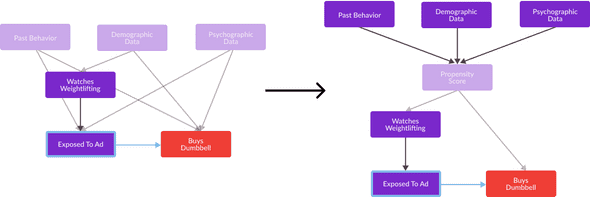
In addition to appropriately choosing features from a set of measured variables, analysts interested in calculating externally valid causal effect estimations must be cautious of features which they did not measure. Consider the digital advertising causal inference task discussed in my previous post. Recall that I used Past Behavior, Demographic Data, and Psychographic Data in order to estimate a propensity score for observed individuals, assuming that these variables comprised all confounding variables affecting both Exposed To Ad and Buys Dumbbell (the pair of variables in the causal relationship I wished to estimate). Recall that I “reframed” my hypothesized causal graph as shown in the figure below in order to effectively control for all confounding.

Figure 1: An illustration of the "reframing" of the causal graph I leveraged in my previous post for propensity score matching. In these causal graphs, the explanatory and outcome variable within my causal effect of interest (which is the effect of Exposed To Ad on Buys Dumbbell) are connected with a blue line. All confounding variables which satisfy a backdoor criterion with respect to these variables are transparent, while all other explanatory variables are opaque. As discussed in my previous post, the main utility of a propensity score is that in a hypothesized causal graph which includes a propensity score, Propensity Score comprises the sole variable within a backdoor admissible set, as displayed in the illustration on the right. As a result, I can achieve an unbiased estimate of my causal effect of interest by controlling solely for Propensity Score.

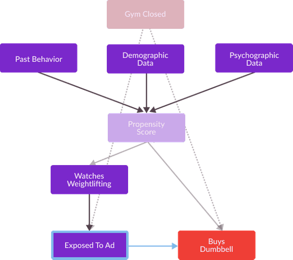
However, what if I didn’t appropriately account for all confounding variables? What effect would that have on the accuracy of my causal effect estimation? Well, suppose there exists an unobserved variable Gym Closed which has an effect on both Exposed To Ad and Buys Dumbbell but is not used to train my propensity score model. Perhaps, whether or not an individual’s local gym is closed has an effect on their inclination to watch weightlifting youtube videos as well as to purchase athletic equipment from my D2C brand. Google provides me with a great deal of demographic information, however highly specific measurements such as Gym Closed is not provided by a generalized digital advertising platform. A causal graph representing this new hypothesized set of causal relationships is as follows.

Figure 2: An illustration of the structural causal model for my digital advertising causal inference task including an unobserved variable Gym Closed which has an effect on both Exposed To Ad and Buys Dumbbell. This illustration highlights the variables which comprise a backdoor admissible set as transparent, while all other variables are opaque. Note that in addition to Propensity Score, Gym Closed is also transparent, implying that I must "control" for this variable in order to achieve an unbiased estimate of the effect of Exposed To Ad on Buys Dumbbell. This will certainly be a challenge, as Gym Closed is unobserved.

Recall that from the definition of blocks on my post on structural causal models, Gym Closed blocks the causal effect between Exposed To Ad and Buys Dumbbell. This means that Gym Closed is a confounding variable, and I must control for it in order to achieve an unbiased estimate of the effect of Exposed To Ad on Buys Dumbbell. Unfortunately, this is impossible as I cannot use any data methodology to make comparisons between Exposed To Ad and Buys Dumbbell while holding Gym Closed constant. In fact, it’s worse than this, I hypothesize that Gym Closed has an effect on both Exposed To Ad and Buys Dumbbell, but I can’t even validate whether or not my hypothesis is correct or not, or whether or not there’s another confounding variable I haven’t accounted for. I don’t know what I don’t know, and what I don’t know can completely invalidate my analysis.

How can I solve a problem I can’t even be sure I have? How do I make sure the propensity score model accounts for all possible confounding variables? There are a few techniques commonly used to mitigate threats to external validity from unmeasured confounding variables.

• Measure everything! A good analyst is biased towards keeping data rather than discarding it, as you may never know what data will be relevant to a subsequent causal effect estimation.
• Leveraging domain expertise in order to exhaust all variables which might affect both an explanatory and outcome variable of interest. Marketers, econometricians, epidemiologists, and physicians rarely select propensity score models features without a depthful qualitative analysis of the confounding variables which must be accounted for during the estimation of a particular causal effect. A systematic approach to feature selection can be crucial for validating that all potential confounding variables have successfully been accounted for.
• Using sensitivity analysis to quantify the extent to which unmeasured confounding may affect the accuracy of an estimation. This can help an analyst understand how different their results would be, given a slight misspecification of their model. I will cover sensitivity analysis techniques for causal inference in more detail in a future blog post.

Propensity Score Balance

Ok, so there are a variety of challenges we can encounter during the first step of propensity score matching, is there anything we must be cautious of after we’ve calculated propensity scores. As you may have guessed: of course there is!

Recall, that the second step of propensity score matching, is the “matching” phase in which an analyst uses an algorithm to identify pairs of one observed and one unobserved individual, in order to subsequently compare each pair’s outcomes while holding their propensity scores constant. Recall from the interactive visualization provided in my previous post, shown again below, only a subsample of observed individuals can be paired to form matched samples.

Note that only a subset of observed individuals can be paired to form matched samples. The only exposed individuals which can be matched by their propensity score to an unexposed individual are those with propensity scores between 0.3 and 0.8. If an exposed individual’s propensity score is less than 0.3, this score is too far away from any unexposed individual for a match to form. Similarly, if an exposed individual’s propensity score is greater than 0.8, this score is too far away from any unexposed individual for a match to form. This phenomenon, in which only a small subset of observed individuals can be matched to unobserved individuals is one of the most significant threats to the external validity of a propensity score matching causal effect estimation for two main reasons.

The first reason that this phenomenon is a threat to external validity is that it results in an insufficient number of matched samples, within a small “matchable” subset. For example, for the data plotted in the interactive illustration above, a propensity score calculation of 32 observed individuals results in only 8 matched samples. If my propensity score calculation avoided this problem, I could’ve made twice as many (16 pairs) from 32 observed individuals, and have had much more evidence of the particular value of a causal effect. A propensity score calculation that is not afflicted by this problem is displayed in the interactive visualisation below.

The second possible threat to external validity encountered after propensity scores have been calculated is a difference in the propensity scores of all observed individuals and the subset of observed individuals which could be matched. Consider again the interactive visualization presented in figure 3. As previously mentioned, only exposed and unexposed individuals in the range of 0.3 and 0.8 are matched in my example dataset, which is starkly different from the range of the set of propensity scores of all individuals (this spans from 0 to 1). In the case of my digital advertising causal inference task, if the set of all individuals I observe during my analysis is representative of all consumers I intend to impact with my advertising decisions, I should be cautious to make decisions based on causal effect estimations derived from such an unrepresentative matched sample. Not all consumers that interact with my brand will have propensity scores in the range of 0.3 and 0.8, so an estimate of the effect of advertising on these individuals is likely quite different than an accurate estimate of the effect of ad exposure on a general population.

Without significant overlap between the propensity scores of individuals exposed and unexposed to treatment, the subsequent matches of these calculated propensity scores will not be large or representative enough to make statistically significant inference of the extent of a causal effect. Balance refers to the extent to which the distributions of propensity scores of individuals exposed and unexposed to treatment overlap. A propensity score calculation is sufficiently balanced if its range of possible matches is large and representative enough to calculate a causal effect estimation which is representative of the outcomes of all observed individuals ². For example, consider the histogram below.

In this histogram, the opaque overlapping region representing the distribution of “matchable” observed individuals is very different from the distributions of individuals exposed and unexposed to treatment. For this reason, this propensity score estimation is unbalanced and an analyst must make some adjustment before interpreting any causal effect estimations leveraging its resulting propensity score match. Below is an example of a histogram displaying the distribution of a balanced propensity score match.

Ok, it’s easy to observe balance as presented with histograms as illustrated above, is there a quantitative way an analyst can measure whether or not a set of propensity score calculations are balanced? Yes! This is commonly done by calculating the standardized mean difference between the propensity scores of the exposed and unexposed treatment groups in order to measure the difference between the means of these distributions in a way that is robust to their respective variation.

Achieving Balance

Equipped with an awareness of the concept of balance and techniques one can use to identify it, how can an analyst ensure that their propensity score model achieves the sufficient balance necessary to make an externally valid causal effect estimation? The main lever analysts have to influence a propensity score calculation is their selection of the confounding variables they use to train their model, and thus, most techniques for improving balance revolve around identifying a subset of confounding variables which optimize this quality. Specifically, these methods select a set of confounding variables with the greatest effect on treatment exposure, as these variables are consequential for ensuring balance of a trained propensity score model ¹. Common causal inference techniques used to select features and ensure balance are as follows:

• Bayesian Additive Regression Trees (BART) Selection Rules, which automatically leverage a machine learning technique for causal inference (BART) to identify the confounding variables which have the greatest effect on exposure to treatment.
• Covariate Balancing Propensity Score (CBPS) a propensity score model which can be used instead of logistic regression in order to model treatment exposure using confounding variables (also known as covariates) which maximize a propensity score’s resulting balance.

What’s Next

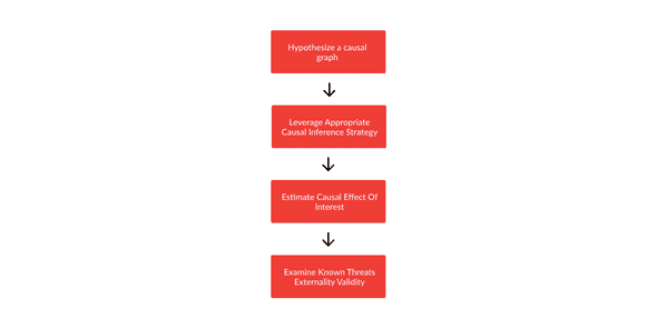
Hopefully, my description of propensity score matching, in this post and my previous one, has given you an introduction to the framework commonly used to analyze techniques designed to solve causal inference tasks. To decide whether or not a particular causal inference technique will accurately estimate a causal effect, an analyst must first understand whether or not this technique is appropriate for the structure of their causal graph. Next, an analyst typically does a “sanity check” of their hypothesis, analuzingThey will then need to analyze a full specification of the technique, in order to ensure they have the appropriate tools to effectively leverage it. Lastly, an analyst will need to understand the common threats to external validity encountered when leveraging this technique, in order to ensure that they are appropriately cautious in their interpretation of any results, and can make any necessary adjustments to calculations in order to achieve an optimally accurate estimate.

Figure 2: An illustration presenting the typical workflow an analysts takes when solving causal inference tasks.

In future blog posts, I will mirror this analytical framework when describing a variety of causal inference techniques. The techniques I will describe span from statistical algorithms, to machine learning applications, to graph-based analytical procedures which can exploit properties of a causal graph. I will discuss how these techniques can help an analyst unlock value from observational data collected in a variety of settings, in order to accurately estimate causal effects with remarkable precision. The description of each technique will be accompanied by a business analytics example for which it is uniquely applicable, as was the case in my presentation of propensity score matching.

I’m excited to continue proselytizing the causal inference literature to curious professionals looking to improve their data-driven decision making capabilities!